Contents
09 May 2025 • 18:10
Trading Simulation with Buy/Sell Signals and Return Percentages
In this article, we are going to simulate a stock market trading strategy using a Random Forest model to predict stock price movements.
Specifically, we will use predictions for when to buy or sell shares, starting with a balance of $10,000. The goal is to evaluate the performance of the strategy over time, tracking both profits and the portfolio’s value.
This article is a continuation of my previous project, where we built a Random Forest model to predict stock price movements based on historical data.
If you’re interested in the details of how the model was trained, feel free to check out the full explanation in my Medium article and the code available on my GitHub repository.
We use a Random Forest model to predict whether the stock price will go up or down, based on features like the Open, Close, Volume, Low, and High prices.
The predictions are used to make simulated buy and sell decisions, applying a transaction fee and tracking the portfolio value over time.
Initial Portfolio: We start with $10,000 in virtual cash.
Buy Decision: We buy the stock when the model predicts that the price will go up.
Sell Decision: We sell the stock when the model predicts that the price will go down.
Transaction Fees: A small fee of 0.1% is applied to both buy and sell actions.
Position Tracking: We track both fractional shares and portfolio value to assess the overall performance.
Below is the code that simulates the stock trading strategy based on the predictions of the Random Forest model.
You can find the complete code in my GitHub repository.
The following code installs the necessary libraries that allow us to retrieve stock data, build plots, and handle model predictions.
%pip install joblib yfinance matplotlib tabulate --quietWe import the libraries we need for data manipulation, visualization, and model prediction.
import joblib
import yfinance as yf
import matplotlib.pyplot as plt
from tabulate import tabulate

plt.style.use("dark_background")
Here, we use joblib to load the trained Random Forest model, yfinance to fetch stock data, matplotlib for visualizations, and tabulate for displaying trading results in a table.
We retrieve the most recent stock data for the company of interest (in this case, Tesla, identified by its ticker symbol TSLA) to simulate the trading strategy.
This is the same company for which the Random Forest model was trained. The data used for simulating the strategy was not part of the training or test set.
The data is downloaded with a weekly interval for analysis similar to the interval used for training.
ticker = "TSLA"
interval = "1wk"

# Load latest data for simulation
df = yf.download(ticker, start="2024-01-01", end="2025-05-08", auto_adjust=True, interval=interval)
df = df[['Open', 'Close', 'Volume', 'Low', 'High']]
df.dropna(inplace=True)
df.head()
Here, we are fetching data for Tesla from January 2024 to May 2025 with a weekly interval.
This code generates a plot of the stock’s closing price over time, allowing us to visualize the stock’s movement.
plt.figure(figsize=(14, 6))
plt.plot(df.index, df["Close"], label="Close", color="blue")
plt.title("Closing Price Over Time")
plt.xlabel("Date")
plt.ylabel("Close Price (USD)")
plt.legend()
plt.grid(True)
plt.savefig("Close.png")
plt.show()
Here, we plot the Closing Price of the stock using matplotlib, which helps to visualize the data and spot patterns or trends.

TSLA Closing Price Over Time
Next, we load the trained Random Forest model using joblib. This model will be used to make predictions based on the features we've prepared.
# Load the model from the file
model = joblib.load('random_forest_model.pkl')

# Use it to make predictions
predictions = model.predict(df)
By loading the trained model, we can now use it to predict whether the stock will go up or down based on the input features.
We add the model’s predictions to the dataset. A Prediction column is created, which indicates whether the model predicts the price will go up (1) or down (0).
# Predict using trained model
df["Prediction"] = model.predict(df)
df.columns = df.columns.get_level_values(0)

df = df[['Open', 'Close', 'Volume', 'Low', 'High', 'Prediction']]
df.head()
The predictions provide us with signals for when to buy (when Prediction == 1) and when to sell (when Prediction == 0).
In this step, we visualize the predicted market direction alongside the stock’s closing price.
# Plotting Close Price and Predictions
plt.figure(figsize=(14, 6))

# Plot the Close Price for the entire period
plt.plot(df.index, df["Close"], label='Close Price', color='blue')

# Plot predicted "Up" signals (where Prediction == 1)
plt.plot(df.index[df["Prediction"] == 1],
         df["Close"][df["Prediction"] == 1],
         '^', markersize=10, color='g', label='Predicted Up')

# Plot predicted "Down" signals (where Prediction == 0)
plt.plot(df.index[df["Prediction"] == 0],
         df["Close"][df["Prediction"] == 0],
         'v', markersize=10, color='r', label='Predicted Down')

# Set the chart title and labels
plt.title("Predicted Market Direction vs Close Price")
plt.xlabel("Date")
plt.ylabel("Close Price ($)")

# Add a legend to differentiate the signals
plt.legend()

# Show grid for better visualization
plt.grid(True)

# Save the plot as a .png file
plt.tight_layout()
plt.savefig("predicted_market_direction.png")

# Display the plot
plt.show()
This plot helps us visually compare the predicted market direction (up or down) against the actual stock price movement.

Predicted Market Direction vs Close Price
This section simulates how the model’s predictions would perform if used in a basic trading strategy.
The logic is straightforward: if the model predicts the stock price will increase the next day, the strategy buys shares; if it predicts a decrease, the strategy sells any shares currently held.
The simulation tracks key metrics including:
Available cash
Number of shares held
Transaction fees
Portfolio value over time
This kind of backtesting allows us to estimate how well our prediction model might perform in a real-world trading scenario.
While it’s a simplified simulation (it doesn’t account for slippage, market spread, or liquidity), it provides a useful benchmark for model performance.
We begin by setting up the initial state for the simulation:
Starting with $10,000 in virtual cash
Holding no shares initially
Keeping a transaction log of each trade
Charging a 0.1% transaction fee per trade (buy or sell)
# Simulate trading strategy
virtual_cash = 10000  # starting balance in dollars
position = 0          # total number of shares held (fractional allowed)
trade_log = []
buy_price = 0         # To track the price at which we bought shares
transaction_fee_percentage = 0.001  # 0.1% fee

# Loop through the data to simulate trading based on predictions
for i in range(len(df) - 1):
    price = df.iloc[i]["Close"]
    next_pred = int(df["Prediction"].iloc[i])  # Predict the action (1 = buy, 0 = sell)

    # Buy if predicted to go up and we have enough cash
    if next_pred == 1 and virtual_cash >= price:
        # Calculate the maximum shares we can buy after accounting for fees
        shares_bought = virtual_cash / (price * (1 + transaction_fee_percentage))
        cost = shares_bought * price
        fee = cost * transaction_fee_percentage
        total_cost = cost + fee

        virtual_cash -= total_cost  # Deduct cost including fee
        position += shares_bought
        buy_price = price

        # Calculate current portfolio value
        portfolio_value = virtual_cash + (position * price)
        trade_log.append(("BUY", df.index[i], price, shares_bought, 0, portfolio_value, fee))

    # Sell if predicted to go down and we hold shares
    elif next_pred == 0 and position > 0:
        proceeds = position * price
        fee = proceeds * transaction_fee_percentage
        net_proceeds = proceeds - fee

        virtual_cash += net_proceeds

        return_percentage = ((price - buy_price) / buy_price) * 100
        portfolio_value = virtual_cash  # After selling, only cash remains
        trade_log.append(("SELL", df.index[i], price, position, return_percentage, portfolio_value, fee))
        position = 0

# Display trade log using tabulate for better visualization
headers = ["Action", "Date", "Price", "Shares", "Return (%)", "Portfolio Value ($)", "Fee ($)"]
print(tabulate(trade_log, headers=headers, tablefmt="grid"))+----------+---------------------+---------+----------+--------------+-----------------------+-----------+
| Action | Date | Price | Shares | Return (%) | Portfolio Value ($) | Fee ($) |
+==========+=====================+=========+==========+==============+=======================+===========+
| BUY | 2024-01-15 00:00:00 | 212.19 | 47.0805 | 0 | 9990.01 | 9.99001 |
+----------+---------------------+---------+----------+--------------+-----------------------+-----------+
| SELL | 2024-04-15 00:00:00 | 147.05 | 47.0805 | -30.6989 | 6916.26 | 6.92319 |
+----------+---------------------+---------+----------+--------------+-----------------------+-----------+
| BUY | 2024-04-22 00:00:00 | 168.29 | 41.0562 | 0 | 6909.35 | 6.90935 |
+----------+---------------------+---------+----------+--------------+-----------------------+-----------+
| SELL | 2024-07-01 00:00:00 | 251.52 | 41.0562 | 49.4563 | 10316.1 | 10.3265 |
+----------+---------------------+---------+----------+--------------+-----------------------+-----------+
| BUY | 2024-07-29 00:00:00 | 207.67 | 49.626 | 0 | 10305.8 | 10.3058 |
+----------+---------------------+---------+----------+--------------+-----------------------+-----------+
| SELL | 2024-09-23 00:00:00 | 260.46 | 49.626 | 25.4201 | 12912.7 | 12.9256 |
+----------+---------------------+---------+----------+--------------+-----------------------+-----------+
| BUY | 2024-10-07 00:00:00 | 217.8 | 59.2276 | 0 | 12899.8 | 12.8998 |
+----------+---------------------+---------+----------+--------------+-----------------------+-----------+
| SELL | 2024-10-21 00:00:00 | 269.19 | 59.2276 | 23.595 | 15927.5 | 15.9435 |
+----------+---------------------+---------+----------+--------------+-----------------------+-----------+
| BUY | 2024-11-18 00:00:00 | 352.56 | 45.1316 | 0 | 15911.6 | 15.9116 |
+----------+---------------------+---------+----------+--------------+-----------------------+-----------+
| SELL | 2024-11-25 00:00:00 | 345.16 | 45.1316 | -2.09893 | 15562.1 | 15.5776 |
+----------+---------------------+---------+----------+--------------+-----------------------+-----------+
| BUY | 2024-12-09 00:00:00 | 436.23 | 35.6383 | 0 | 15546.5 | 15.5465 |
+----------+---------------------+---------+----------+--------------+-----------------------+-----------+
...
| SELL | 2025-03-10 00:00:00 | 249.98 | 47.2332 | -14.6768 | 11795.5 | 11.8074 |
+----------+---------------------+---------+----------+--------------+-----------------------+-----------+
| BUY | 2025-04-28 00:00:00 | 287.21 | 41.0284 | 0 | 11783.8 | 11.7838 |
+----------+---------------------+---------+----------+--------------+-----------------------+-----------+This simulation executes a simple, rule-based strategy:
Buy if the model predicts an upward movement and we have enough cash
Sell if the model predicts a drop and we’re holding any shares
At each step, the portfolio value is updated and the transaction (with fee and returns) is logged
After simulating the sequence of trades, we calculate the final portfolio value to assess the performance of the strategy over time.
# Calculate final portfolio value and return percentage
final_price = df.iloc[-1]["Close"]  # Last closing price
final_value = virtual_cash + (position * final_price)  # Final value of portfolio
profit = final_value - 10000  # Profit or loss from initial investment
return_percentage = (profit / 10000) * 100  # Return as percentage

# Print final results
print(f"Final Portfolio Value: ${final_value:.2f}")
print(f"Profit/Loss: ${profit:.2f}")
print(f"Return: {return_percentage:.2f}%")Final Portfolio Value: $11685.71
Profit/Loss: $1685.71
Return: 16.86%This step provides a snapshot of the strategy’s outcome:
Final portfolio value includes both remaining cash and the market value of any unsold shares.
Profit/Loss is computed relative to the initial capital.
Return percentage reflects the overall profitability of the strategy.
To gain further insight into how the portfolio performed throughout the simulation, we plot the portfolio value after each buy or sell decision.
# After the trading loop
portfolio_values = [trade[5] for trade in trade_log]
dates = [trade[1] for trade in trade_log]

# Plot portfolio value over time
plt.figure(figsize=(14, 6))
plt.plot(dates, portfolio_values, label="Portfolio Value", color="purple")
plt.title("Portfolio Value Over Time")
plt.xlabel("Date")
plt.ylabel("Portfolio Value ($)")
plt.grid(True)
plt.tight_layout()
plt.savefig("portfolio_value_over_time.png")
plt.show()
Portfolio Value Over Time
Beyond raw returns, it’s important to evaluate how efficiently the strategy generated returns relative to the volatility of outcomes. We compute the Sharpe Ratio for this purpose.
# After final portfolio value is printed
returns = [trade[4] for trade in trade_log if trade[4] != 0]
mean_return = sum(returns) / len(returns)
stddev_return = (sum([(r - mean_return)**2 for r in returns]) / len(returns))**0.5
sharpe_ratio = mean_return / stddev_return if stddev_return != 0 else 0
print(f"Sharpe Ratio: {sharpe_ratio:.2f}")Sharpe Ratio: 0.20Finally, we overlay buy and sell signals on the closing price chart, showing exactly when trades occurred and the returns achieved on each.
# Plotting Buy/Sell signals on Close price
plt.figure(figsize=(14, 6))
# Plot the Close Price with a lower zorder
plt.plot(df.index, df["Close"], label="Close Price", color="blue", zorder=1)
# Plot Buy and Sell signals with a higher zorder
for action, date, price, shares, return_pct, portfolio_value, fee in trade_log:
if action == "BUY":
# Scatter plot for Buy signal
plt.scatter(date, price, marker='o', color='orange', s=100, label="Buy Signal" if 'Buy Signal' not in plt.gca().get_legend_handles_labels()[1] else "", zorder=2)
plt.annotate(f"BUY", (date, price), textcoords="offset points", xytext=(0, 10), ha='center', fontsize=10, color='orange', zorder=3)
else:
return_color = 'lime' if return_pct > 0 else 'red' # Green for positive return, red for negative
# Scatter plot for Sell signal
plt.scatter(date, price, marker='v', color=return_color, s=100, label="Sell Signal" if 'Sell Signal' not in plt.gca().get_legend_handles_labels()[1] else "", zorder=2)
# Annotate with return percentage (if available)
plt.annotate(f"SELL \n {return_pct:.2f}%", (date, price), textcoords="offset points", xytext=(0, -30), ha='center', fontsize=10, color=return_color, zorder=3)
# Set chart title and labels
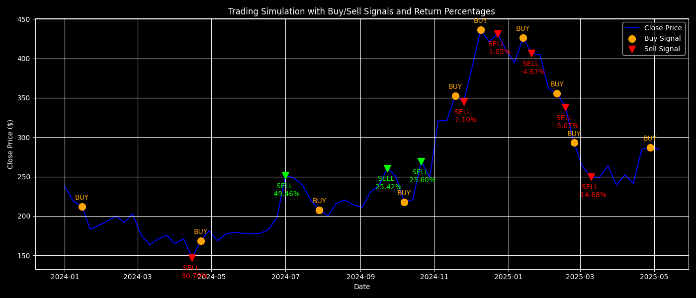
plt.title("Trading Simulation with Buy/Sell Signals and Return Percentages")
plt.xlabel("Date")
plt.ylabel("Close Price ($)")
# Add legend
plt.legend()
# Add grid for better visualization
plt.grid(True)
# Tight layout to avoid clipping
plt.tight_layout()
# Save and display the plot
plt.savefig("trading_simulation_2024_2025_with_return.png")
plt.show()Trading Simulation with Buy/Sell Signals and Return Percentages
This annotated plot adds interpretability to the model’s predictions:
Orange dots indicate buy signals.
Green/red triangles show sell decisions and highlight positive or negative returns respectively.
Annotations give context for each action, showing not just timing but also impact.
Thank you for reading this article and following along with the trading simulation. I hope you found this insightful and helpful for your journey into algorithmic trading.
You can access the full code for this simulation, along with other related resources, on my GitHub repository. Also check out the following article on How we trained the random forest model.


